

Forecast methods
The first purpose of the forecast module is to compute statistical forecast based on the demand history. FrePPLe implements 5 times series methods to compute the statistical forecast.
Check this feature on a live example
Download an Excel spreadsheet with the data for this example
Let’s review these forecasting methods in an example:
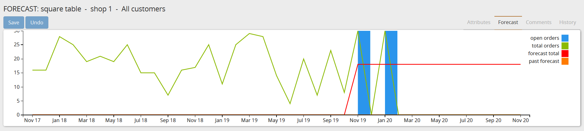
- Moving average:This method simply calculates the average of the demand history for the last N time buckets where N is a configurable parameter (see parameter forecast.MovingAverage_order).In real-life datasets you will normally only see this method being selected when there is only very limited history (eg a new item).
- Constant:The constant method is an implementation of the single exponential smoothing method. It is used when the demand doesn’t really evolve in time.
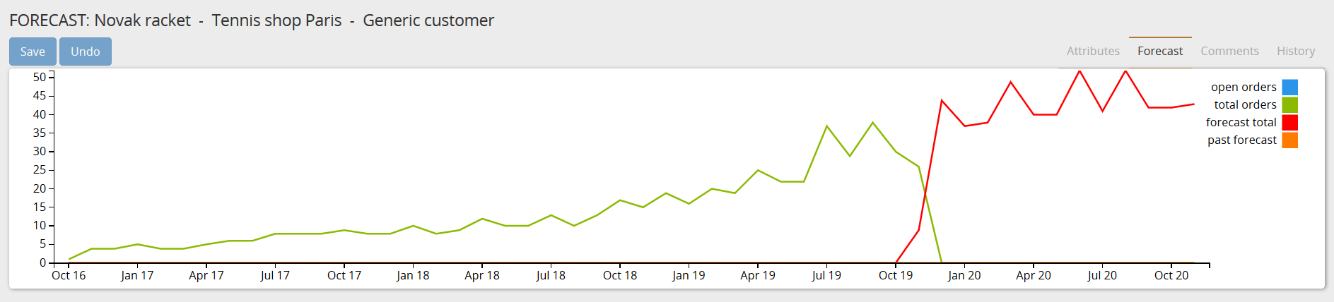
- Trend:The trend method is an implementation of the double exponential smoothing method. It is used when a trend, either positive or negative, is observed in the sales history.
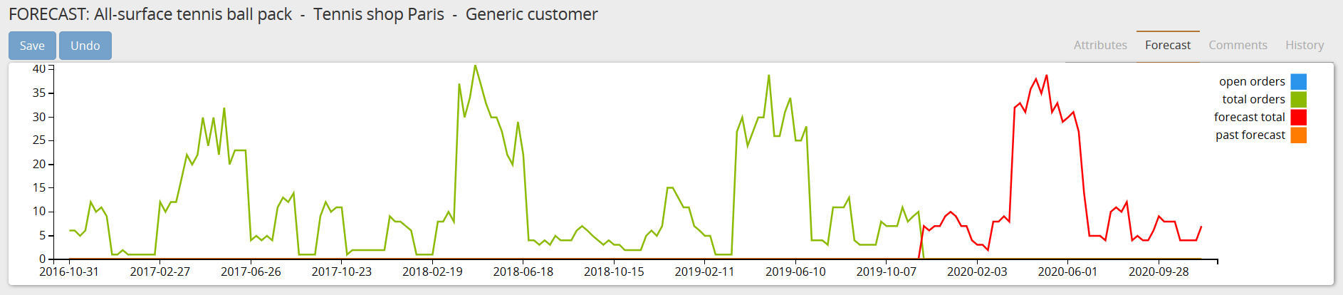
- Seasonal:The seasonal method is an implementation of the Holt-Winter’s method and is used when a seasonal pattern is detected in the demand history.A seasonal forecast has a recurring pattern in time such as ice creams being much more sold during summer compared to winter.FrePPLe automatically detects for the periodicity of the recurring patterns.
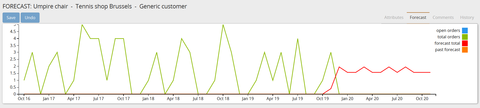
- Intermittent:The intermittent method is an implementation of the Croston method. This method is suitable for sales history with intermittence, i.e. a sales history with many zeros.
The forecast module also provides 3 other options to compute the statistical forecast:
- Automatic (default):This is the default forecast method. FrePPLe will evaluate all 5 statistical forecast methods described above and will pick the one that minimizes the forecast error.
- Manual:This option prevents frePPLe from computing any forecast. The forecast will be provided by the planner through overrides.
- Aggregate:It means that the forecast should be equal to the sum of the child intersections’ forecast. This method is automatically set on all parent nodes in the hierarchy.
Follow these steps to explore this example in more detail:
- The forecast table contains the intersections for which a forecast should be computed.By default, this table is automatically populated based on the intersections found in the demand history (see the parameter forecast.populateForecastTable for more details).Using the “method” field in the forecast table you can choose among the different methods. By default the method will be set to “automatic”.
The forecasts are best navigated with the forecast report or the forecast editor