
Demand classification
Why forecastability matters
Have you noticed that, for some products, you just never seem to reach your forecast accuracy objectives? Have you had to relentlessly explain to your management that you can’t do better?
Let us make your day: it’s not your fault. It really isn’t. Here, the metric is to blame.
Indeed, your forecast accuracy strongly depends on your product forecastability. We can find evidence of it in your demand history characteristics.
To determine a product forecastability, we apply two coefficients:
- the Average Demand Interval (ADI). It measures the demand regularity in time by computing the average interval between two demands.
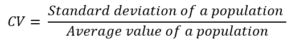
- the square of the Coefficient of Variation (CV²). It measures the variation in quantities.
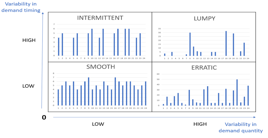
Based on these 2 dimensions, the literature classifies the demand profiles into 4 different categories:
- Smooth demand (ADI < 1.32 and CV² < 0.49). The demand is very regular in time and in quantity. It is therefore easy to forecast and you won’t have trouble reaching a low forecasting error level.
- Intermittent demand (ADI >= 1.32 and CV² < 0.49). The demand history shows very little variation in demand quantity but a high variation in the interval between two demands. Though specific forecasting methods tackle intermittent demands, the forecast error margin is considerably higher.
- Erratic demand (ADI < 1.32 and CV² >= 0.49). The demand has regular occurrences in time with high quantity variations. Your forecast accuracy remains shaky.
- Lumpy demand (ADI >= 1.32 and CV² >= 0.49). The demand is characterized by a large variation in quantity and in time. It is actually impossible to produce a reliable forecast, no matter which forecasting tools you use. This particular type of demand pattern is unforecastable.
For all but the smooth demand profile, forecast accuracy is not a reliable performance metric. It lacks contextual information and, in the end, leads you to miss the big picture.
This induces overstock situations or, on the contrary, poor service level, both situations you want to avoid.
This is why you should take some time to understand your products’ various demand patterns, step back, and adjust your expectations. Virtually all companies can find products in each of the 4 categories: smooth, intermittent, erratic, or lumpy demand.
Details of the math
To better understand these two coefficients, let’s take an example of a demand history over twelve time buckets:
| Period | 1 | 2 | 3 | 4 | 5 | 6 | 7 | 8 | 9 | 10 | 11 | 12 |
| Demand Quantity | 6 | 5 | 9 | 2 | 14 | 21 | 17 |
The ADI is equal to the average interval between two demands:
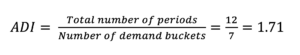
We can say that, in our data sample, a demand occurs on average every 1.71 periods.
The CV² is defined as the square of the CV, the coefficient of variation.
To compute the coefficient of variation, we are only considering the non-zero values of the demand history. In our sample, the average quantity is 10.57, while the standard deviation is 6.43. Therefore, we can deduce the CV²:
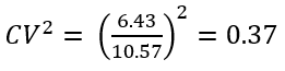
This is an intermittent demand pattern.
Concrete case
For the sake of the exercise, let’s compute the ADI and CV² for a large group of products.
Here, we used another data sample and displayed the results in a scatter plot to identify general characteristics.
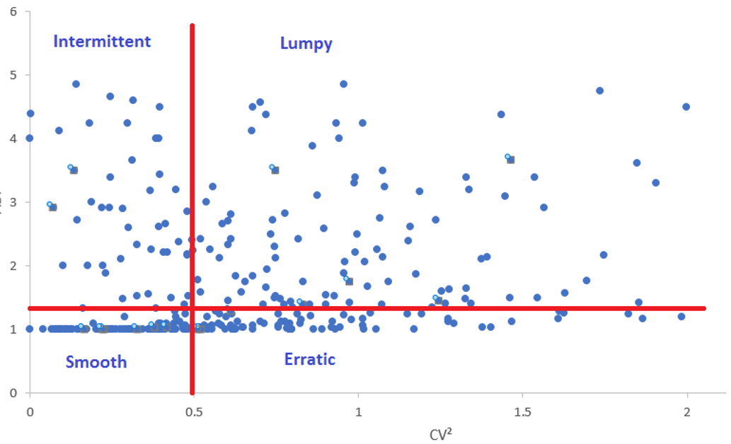
If we sum up the number of points per demand profile, we have:
| Demand Profile | Number of parts | Percentage |
| Smooth | 92 | 23% |
| Erratic | 97 | 24% |
| Intermittent | 67 | 17% |
| Lumpy | 147 | 36% |
In the above example, 23% of the products have a smooth demand history profile, meaning that they should be easy to forecast. 40% of them are either erratic or intermittent and forecasting them is already more difficult. For the remaining 36%, the lumpy ones, we won’t reach an accurate forecast.
With this distribution pattern, we can conclude that the management of this company should focus on the safety stock and service levels to cover for the variable nature of their demand rather than aiming at improving the forecast accuracy.
Understanding a product forecastability is a must to set correct anticipations on what you can achieve in terms of forecast accuracy. In the end, it is not about reaching the highest accuracy, it is about being able to answer customer demand when it hits.
When you upload your demand history into frePPLe, the algorithm automatically detects the demand pattern for each item (i.e. product or SKU), as shown below. When you plan your forecast, you can expect a higher standard deviation for intermittent, erratic, and lumpy items.
Ultimately, this allows you to adjust your expectations and explain to your manager — with hard data — why the forecast accuracy might not be that good for these specific items, and how you can adapt to this parameter by raising your service level.
Curious about the forecastability of your data ? You can download frePPLe and give it a try. The forecasting module is 100% free and open source.
Find out more about the demand forecasting module and how to optimize your inventory.
For more information, contact us.