Forecast methods

The first purpose of the forecast module of frePPLe is to compute statistical forecast based on the demand history. The forecast table of FrePPLe contains the intersections for which a forecast should be computed. By default, this table is automatically populated by frePPLe based on the intersections found in the demand history (see parameter forecast.populateForecastTable fore more details). The forecast table contains a field named method where the planner can choose among different methods which one should be picked by frePPLe. FrePPLe proposes 5 textbook methods to compute the statistical forecast.

Example

Excel spreadsheet forecast-method

1. Moving average: This method simply calculates the average of the demand history for the last n time buckets where n is a configurable parameter (see parameter forecast.MovingAverage_order). This method could be seen as the default method when no other method applies.
2. Constant: The constant method is an implementation of the single exponential smoothing method. It should be used when the demand history doesn’t really evolve in time.

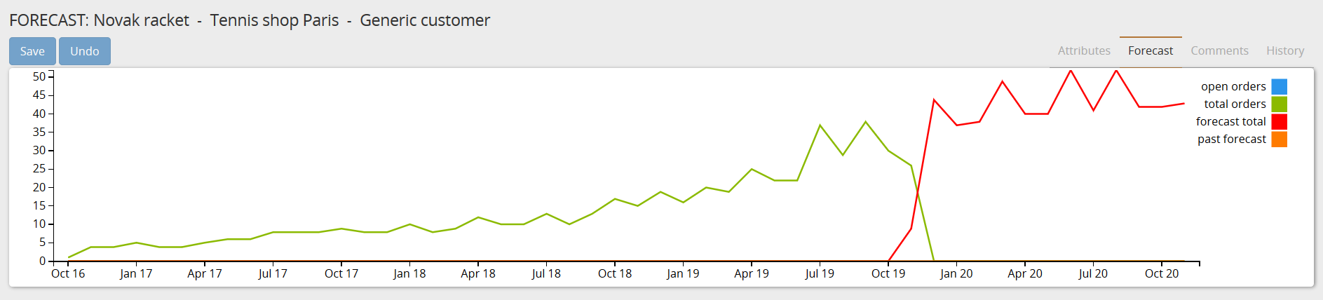
3. Trend: The trend method is an implementation of the double exponential smoothing method. It should be used when a trend, either positive or negative, is observed in the sales history. The trend method will be used on a demand history like this:

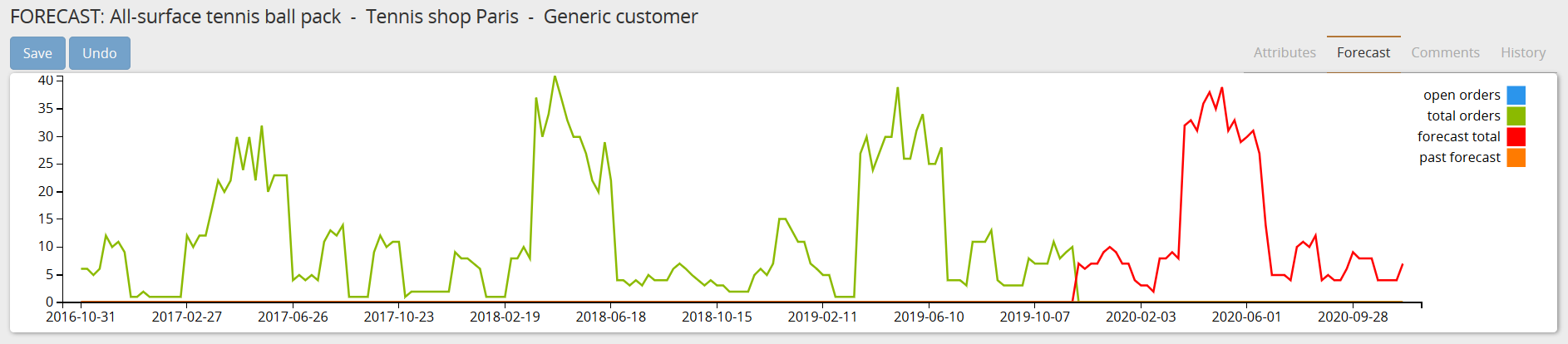
4. Seasonal: The seasonal method is an implementation of the Holt-Winter’s method and should be used when seasonality applies ot the demand history. A sesasonal forecast has a recurrent pattern in time such as ice creams being much more sold during summer compared to winter. Note that if the seasonal method is set for a given combination and the forecast solver is unable to find any seasonality pattern then it will revert to moving average. The seasonal method will be used on a demand history like this:

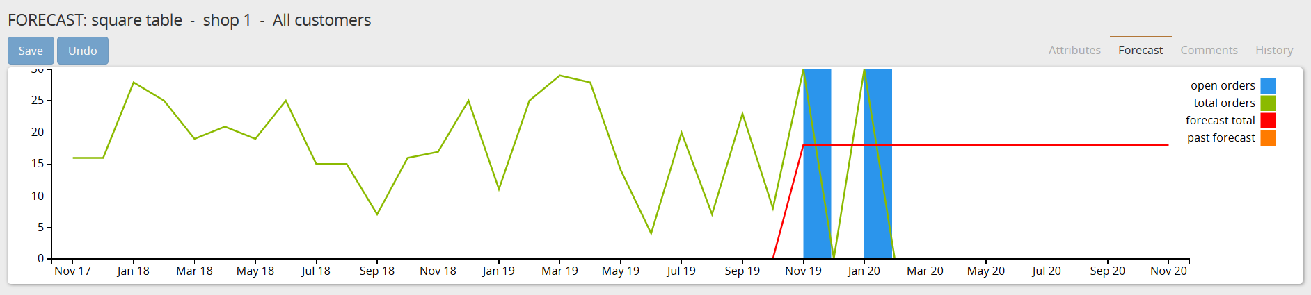
5. Intermittent: The intermittent method is an implementation of the Croston method. This method is suitable for sales history with intermittence, that is when some periods with no demand history are followed by periods with demand history. An intermittent demand history will look like this:

For advanced users, each of the above methods has specific parameters in the parameter table that can be tuned to adjust the forecast results.

The forecast module also provides 3 other options to compute the statistical forecast:

1. Automatic: This option is the one by default. FrePPLe will test all 5 statistical forecast methods described above and will pick the one that minimizes the forecast error. Note that the solver used in frePPLe will also tune each method parameters (defined with a minimum and amximum value) to try to find the parameters that minimize the demand history (see parameter forecast.Iterations).
2. Manual: This option prevents frePPLe from computing any forecast. This option should be chosen when the forecast will be provided by the planner through overrides.
3. Aggregate: It means that the forecast should be equal to the sum of the child intersections’ forecast. This option is deprecated as all parent intersections are automatically calculated without having to specify a record in the forecast table for the parent.

In below Excel file, we have shrunk the distribution demo model to keep four intersections where the constant, trend, intermittent and sesasonal methods have been picked.