A previous article explained why inventory is stored at decoupling points in your supply chain.

We also explored the topic of demand variability, demand patterns and their implications.

A logical next question is “how much inventory do you need at a decoupling point to protect against the variability?”
Let’s expand on this subject step by step and learn the art and science of computing safety stocks.

Step 1: Determine the demand and its variability

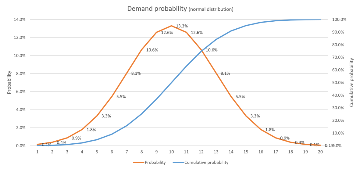
A first step in any safety stock calculation is to measure the demand variability. Demand is not constant over time, and the demand per time bucket (either day, week or month) will have a certain statistical distribution.

In most cases a normal distribution is appropriate. In fact, many textbook safety stock formulas always assume a normal distribution.
For slow moving items (such as spare parts), a Poisson distribution is a more accurate representation of the underlying demand.
And for erratic and bulky demand patterns other distributions such as negative binomial can be applied.

The estimation of the demand variability should only consider unexpected variations. Known exceptional demands (aka outliers) should be excluded. For seasonal items, the estimated variability should filter out the normal seasonal changes. Similarly, for trending items the trend component should be filtered out. In other words, measuring the demand variability is a bit more complex than computing the standard deviation of the demand per time bucket.

The image below shows the demand per bucket for a normal distribution with average 10 and standard deviation 3. On average the demand is 10. In 8.1% of buckets the demand will only be 7. And in 3.3% of buckets the demand will be 15.

Step 2: Determine the lead time and its variability

The safety stock increases with the lead time. During replenishment lead time we can’t react to unexpected changes. The longer the lead time, the longer the period during which we rely solely on the safety and existing open replenishment to cover the variability.

See this article on the determination of the decoupled lead time. For a purchased item, it’s the purchasing lead time. For a manufactured item it’s the longest chain of production times between decoupling points.

Variability in the lead time is measured by analyzing the standard deviation of the transaction history. This calculation isn’t easy, even from the transaction data in the most advanced ERP systems. In practice, most companies will either ignore this variability or use a few categories (such as “low supply variability”, “medium supply variability”, “high supply variability”) and rules of thumb to estimate the supply variability.

Step 3: Determine the required service level

Safety stocks aren’t an absolute protection against stockouts. A safety stock is always a balance between the risk and impact of a stockout and the cost of the extra safety stock inventory.
The service level captures this balance. The service level is the percentage of the demand quantity you will be able to honor from your inventory.

For critical items, you want to be more than 99.x% sure you have them on stock when a demand comes in.

For a less critical items, you can can accept a stockout risk that is be considerably higher. Either the customer will wait during a temporary stockout, either you accept missing a small part of sales.

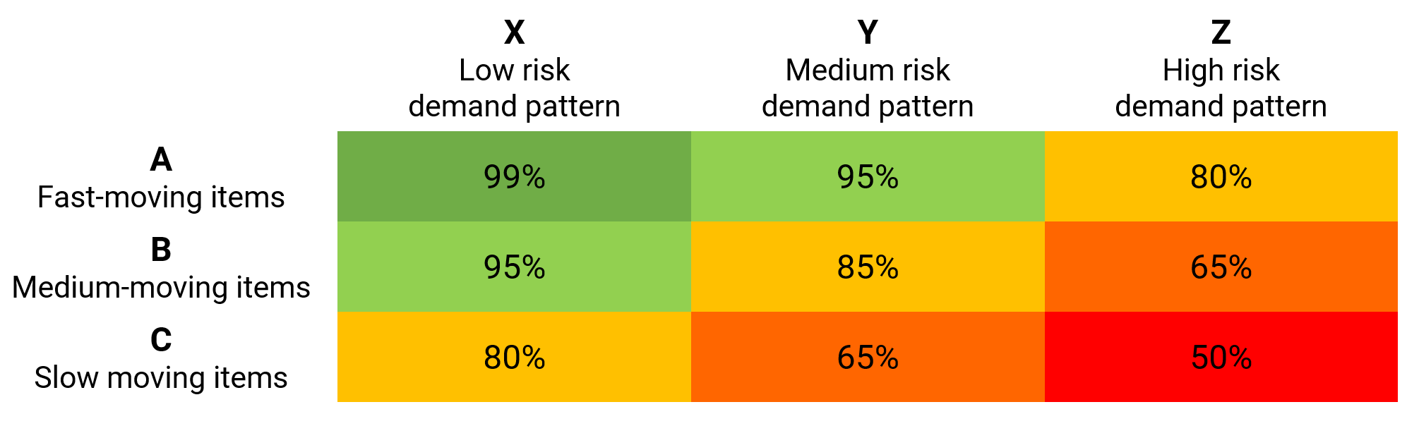
A ABC or ABC-XYZ analysis of your products is very common to choose an appropriate service level.  The picture below shows an example of such a matrix. The matrix varies greatly by industry and company: a supermarket will operate with a completely different set of rules and objects than a spare parts warehouse or a industrial equipment manufacturer.

Step 4: Computing the safety stock

Putting all the above together, we can now compute the safety stock.

We go through the following steps:

• The distribution from step 2 measures the demand variability for a single time bucket.
  It is extended to a) cover the complete lead time, and b) include the lead time variability.
• We generate a graph of the cumulative probability.
• In this graph, we can easily look up the safety stock that will provide us the desired service level.
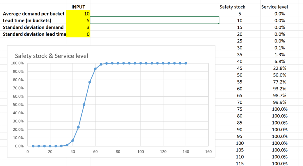
  The picture below shows this graph for the same example item we used before. The total demand during the lead time is 5 * 10 = 50 units.
  In the picture below we find that a safety stock of 50 units gives us a service level of 50%.
  We find that a safety stock of 60 units already gives us a service level of 93%.
• Notice how the graph is very flat when we go to very high service levels. Service levels > 99.x will turn out to be very expensive inventory decisions.

Here is an excel spreadsheet where you can play around with different values.

Step 5: Practical considerations and constraints

We’re not done yet. Computing safety stocks is both an art and a science. You’ve learned the science part now. It’s time to bring in the art component. This is where the planners judgement and experience plays an important role.

The outcome of the above calculation can’t be taken for granted in all situations. Some examples:

• For products with a limited lifetime we need to assure that we don’t stock the product for too long.  The safety stock and reorder quantity need to be low enough to avoid inventory going obsolete.
• Some items may be so critical or strategic to your business that you want to impose a minimum safety stock that exceeds the outcome of the formula.
  Eg In some countries petroleum companies are legally obliged to maintain a strategic stock at all times.
  Eg Certain spare parts for an airplane are categorized as aircraft-on-ground critical. When such a part is broken the plane simply can’t fly safely and will be kept on the ground.  Manufacturers of such parts will set apart a certain stock to respond to emergencies on such items.
• In practice the outcome of the safety stock formula can be quite abstract. When the outcome is expressed in terms of the number of days of demand it covers, we obtain a metric that is understood more intuitively by planners.
  It’s not uncommon to define safety stocks as a period of cover, or to impose a minimum or maximum days of cover limit to the outcome of the safety stock formula.
• The formula assumes the lead time is a hard limit (i.e. changing the replenishments within the lead time isn’t possible). In practice it is often possible to expedite purchase orders or manufacturing orders. The lead time and/or the service level for the formula should reflect this.

In summary, there is more than enough room where rules of thumb and the planner’s interpretation and experience comes into the picture. After all, a safety stock is a balanced inventory risk decision that goes deeper than any mathematical formula.